In this first project of 2022, I will be fitting linear and polynomial regression models to some randomly generated dataset where there is a nonlinear relationship between the target and the predictor.

The purpose of this project is to observe some of the red flags for a model that is severely underfitting to the data and how these red flags change when fitting a more appropriate model.

The red flags that I’ll be considering are:

• MSE and R-squared – these are common performance metrics used in linear models.
• Residual plot – this plot will show us if some of the assumptions of linear regression have been violated.
• Learning curves – this plot will show us how well the model fits to the data and usually gives a good indication of over/under fitting.

Generating the data

I generate the data using a polynomial equation of degree 2:

# Generate some nonlinear data
m = 500
X = 9 * np.random.rand(m, 1) - 1
Y = 0.5 * X**2 - 3 * X + 7 + np.random.randn(m, 1)

In this visualisation of the data, we can clearly see the nonlinear relationship that we have generated from the above equation:

Linear Regression

Being one of the oldest and simplest models, linear regression is pretty well known and easy to understand. In this project, I am using linear regression to demonstrate what underfitting looks like and as a comparison to polynomial regression.

To fit linear regression, the response variable must be continuous. There are also a couple of assumptions that must be satisfied in order to use linear regression with some degree of accuracy, otherwise the results can be misleading or downright incorrect.

• Linearity: the relationship between the response variable and the predictors must be linear.
• Homoscedasticity: the variance of the residuals must be constant. So, as the value of the predictor increases, the variability in the response stays the same.
• Independence: the residuals must be independent of one another. This means that each observation must not be determined by or correlated with another. Usually only an issue in time series data.
• Normality: the residuals are normally distributed. In other words, the average of all residual values is zero.

These assumptions are usually overlooked when linear regression is applied but they are very important. In this project, The assumptions of linearity and normality are both purposely violated to support the decision to use polynomial regression.

Below is the linear regression model fitted to the generated dataset:

linear_regressor = LinearRegression()
linear_regressor.fit(X_train, Y_train)

Y_predict = linear_regressor.predict(X_test)
linear_mse = mean_squared_error(Y_test, Y_predict)
print(f"MSE (linear regression): {round(linear_mse,2)}")

linear_r2_score = r2_score(Y_test, Y_predict)
print(f"R2 Score (linear regression): {round(linear_r2_score,2)}")

This model gives a Mean Square Error (MSE) score of 10.0 and an R-Squared (R2) score of 0.27. Both these scores give our first red flags. Ideally, MSE should be as low as possible (around 1 is very good) and R-squared should be as close to 1 as possible. So far, our model is not doing a good job of describing the data.

Let’s plot the residuals versus the fitted values – this gives a good indication of whether the assumptions of linearity and normality are violated. Ideally, there should be a random scatter of points around 0 with no discernible pattern or shape in the data. The below plot shows a definite nonlinear pattern in the data:

Next is the learning curves. To generate this plot, multiple models are fitted to varying dataset sizes and the Root Mean Square Error (RMSE) is recorded. In this plot, we get to compare the training performance against some predictions made on a validation set.

As before, we want the RMSE to be as low as possible. But now, we also want the training and validation errors to be as close as possible as the training set size increases. If the validation error is higher than the training error then we know that the model did not generalise well to new data and this is a red flag for over/under fitting.

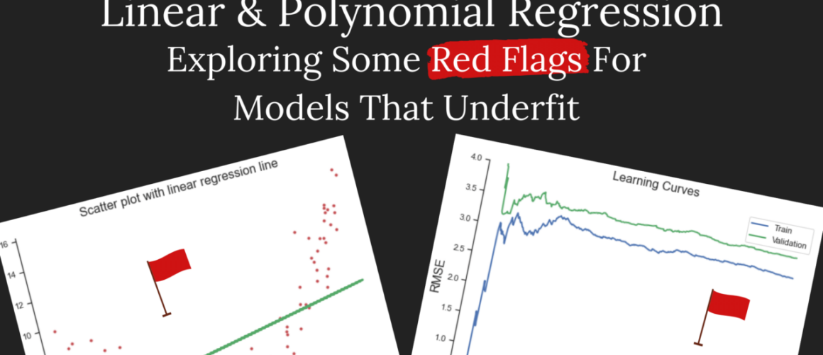
In these learning curves for linear regression, not only is the RMSE high, but the validation error remains higher than the training error throughout the process.

Great, so now that we know that that above model is a total mess and does a really bad job at making predictions, let’s make a better choice.

Polynomial Regression

When the assumptions of linear regression are not satisfied and the model isn’t capturing the relationship between the response and the predictors then we need a different approach.

Polynomial regression lets us model a non-linear relationship between the response and the predictors. It is a natural extension of linear regression and works by including polynomial forms of the predictors at the degree of our choosing.

polynomial_features = PolynomialFeatures(degree = 2, include_bias = False)
X_train_poly = polynomial_features.fit_transform(X_train)
X_test_poly = polynomial_features.fit_transform(X_test)

linear_regressor = LinearRegression()
linear_regressor.fit(X_train_poly, Y_train)

Y_predict_poly = linear_regressor.predict(X_test_poly)
poly_mse = mean_squared_error(Y_test, Y_predict_poly)
print(f"MSE (polynomial regression): {round(poly_mse,2)}")

poly_r2_score = r2_score(Y_test, Y_predict_poly)
print(f"R2 Score (polynomial regression): {round(poly_r2_score,2)}")

Here, we get a wonderful MSE score of 1.0 and an even better R-squared score of 0.9. Plotting the new polynomial regression line to our data we see that it fits like a glove:

Plotting residuals versus fitted values again we now see that there is a nice random scatter of points around 0 and I can’t make out any patterns, so that’s good!

Lastly, the learning curves. Both the validation and training errors hover at around 1.00 and although the lines do not meet in this plot, if I added more data, they would eventually converge.

I hope this project gave you some insight into the red flags commonly seen for linear models that underfit. Reach out to me on Twitter if you have any feedback or questions.

You can find the full code for this project on GitHub.